Variational Auto-encoders

Autoencoders learn low-dimensional representation of the data in unsupervised way by aiming to imitate the identity function i.e. reconstruct the original data while having a low-dimensional representation bottleneck in the process. In other words, Autoencoders are neural networks trained to generate output y that is as close to the input x, and an internal layer that gives the representation z(x) for each new input.

Composed of two networks:

• Encoder $E_{\theta }:\mathcal{X}\to \mathcal{Z}$: Maps high-dimensional input to low-dimensional latent representation, usually $|\mathcal{Z}|\le |\mathcal{X}|$.
• Decoder $D_{\varphi }:\mathcal{Z}\to \mathcal{Y}$: Outputs data as close to original from latent representation.

Encoder network is generally used to accomplish dimensionality reduction when $|\mathcal{Z}|\ll |\mathcal{X}|$ and can be seen as a non-linear generalisation to PCA.

Deterministic AE

• Denoising AE
• Sparse AE
• Contractive AE

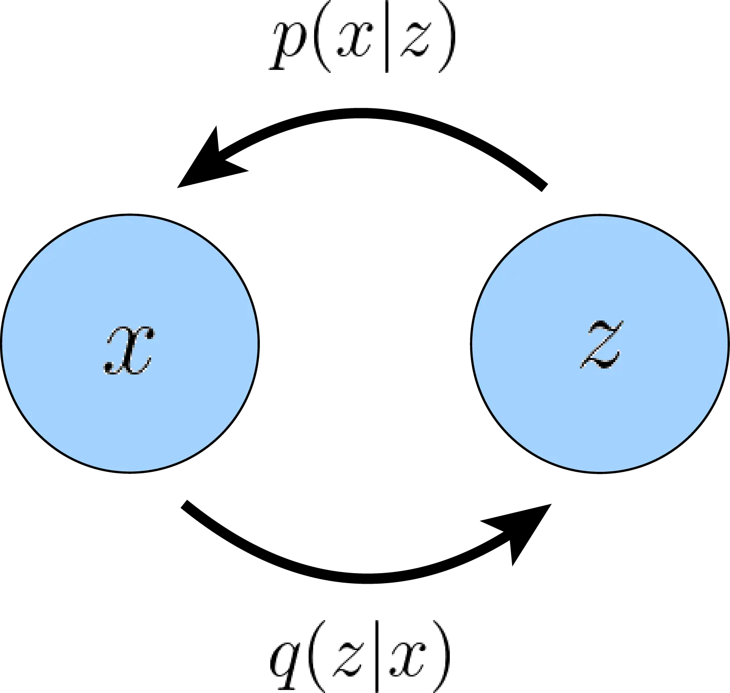
Consider random variables x and z, with g being deterministic decoder (generator) and f being deterministic encoder. The process looks like:

\begin{array}[cc] \\ \mathbf{x}\sim p_{\mathcal{D}} & \mathbf{z}\sim p_{\mathbf{z}} \\ \hat{\mathbf{z}}=f(\mathbf{x}) & \hat{\mathbf{x}}=g(\mathbf{z}) \end{array}

Our goal is to generate $\mathbf{x}$ or in other words sample $\mathbf{x}$ from distribution $p_{\theta }(\mathbf{x})$. If we know the distribution to latent variable z, then expressing x is just taking marginal likelihood $p_{\theta }(\mathbf{x})={\int }_{\mathbf{z}}{p}_{\theta }(\mathbf{x}|\mathbf{z})p(\mathbf{z})d\mathbf{z}$ over latent variables $p(\mathbf{z})$ with the conditional distribution of $p_{\theta }(\mathbf{x}|\mathbf{z})$, or if we have access to ground truth latent encoder, we can also write $p(x)=\frac{p(x,z)}{p(z|x)}$

Using log likelihood objective ${\sum }_{i=1}^N\log p_{\theta }({\mathbf{x}}^{(i)})$, we can optimise $\theta$ by minimising the NLL.

But generally, z is not known, and primary goal of a generative model is to create output from scratch. So, we need a distribution $p_{\mathbf{z}}$ so that z can be sampled from the distribution. You might ask, why can’t an AE be used for this, where we can use the encoder to get the sample z? Firstly, encoder works on an input, and secondly, is optimised to work as a identity lookup table. The latent space might not be structured, and AE doesn’t provide any guarantee about the structure of the latent variable distribution.

To calculate the intractable data likelihood $p_{\theta }(\mathbf{x})$, we make following assumptions:

1. Hypothesis space $p_{\theta }(\mathbf{x}|\mathbf{z})$ is modelled using a product mixture of distributions (e.g., Gaussians or Bernoullis) with a prior $p_z$ (usually Gaussian). Thus, VAEs can be seen as an infinite mixture of Gaussians. To prevent learning infinite set of parameters over discrete latent space, VAE uses a function $g_{\theta }$ that outputs the parameters of a continuous latent variable, and smoothens the latent space.

$$p_{\theta }(\mathbf{x})={\int }_z\mathcal{N}(\mathbf{x};g_{\theta }^{\mu }(\mathbf{z}),g_{\theta }^{\Sigma }(\mathbf{z}))\mathcal{N}(\mathbf{z};0,I)d\mathbf{z}$$

2. Importance sampling using another density $z\sim q_z$. Instead of approximating the integral over all z (because most of the term will be near zero), we want to sample z from the distribution $p_{\theta }(z|x)$ whose sample places maximum likelihood on x $p_{\theta }(x|z)$. Optimal $q^{\ast }=p_{\theta }(\mathbf{z}|\mathbf{x})$.

$$p_{\theta }(\mathbf{x})=E_{z\sim p_z}[p_{\theta }(\mathbf{x}|\mathbf{z})]={\int }_z{q}_{\mathbf{z}}(\mathbf{z})\frac{p_{\mathbf{z}}(\mathbf{z})}{q_{\mathbf{z}}(\mathbf{z})}{p}_{\theta }(\mathbf{x}|\mathbf{z})d\mathbf{z}=E_{\mathbf{z}\sim p_{\mathbf{z}}}[\frac{p_{\mathbf{z}}(\mathbf{z})}{q_{\mathbf{z}}(\mathbf{z})}{p}_{\theta }(\mathbf{x}|\mathbf{z})]$$

3. Use variational inference to estimate p by modelling $q_{\varphi }$ parametrised by $\varphi$. Posterior distribution $q_{\varphi }(\mathbf{z}|\mathbf{x})=\mathcal{N}(f_{\varphi }^{\mu }(\mathbf{x}),f_{\varphi }^{\Sigma }(\mathbf{x}))$ uses approximation function $f$ that outputs the parameters of the distribution and can be seen as probabilistic encoder.

Our goal will be to use the representation of the distribution $p(x)$ to derive a term called the Evidence Lower Bound (ELBO), which gives a lower bound on the evidence. Evidence is written as log likelihood of the observed data: $\log p(\mathbf{x})$. ELBO gives a proxy objective that can be optimised with respect to a latent variable model, and in the best case (when true distribution is learned), ELBO exactly equals the evidence.

Objective

The estimated posterior $q_{\varphi }(\mathbf{z}|\mathbf{x})$ needs to be close to best approximation $p_{\theta }(\mathbf{z}|\mathbf{x})$, and is measured using reversed KL divergence $D_{\text{KL}}(q_{\varphi }(\mathbf{z}|\mathbf{x})\Vert p_{\theta }(\mathbf{z}|\mathbf{x}))$.

Why use reverse KL?

Doesn’t KL $D(p\Vert q)$ measure how many bits is required to estimate p using q? Then, why are measuring how many bits are required to go from p to q, when instead we are approximating p with q?

$$\begin{array}{rlr}{D}_{\text{KL}}(q_{\varphi }(\mathbf{z}|\mathbf{x})\Vert p_{\theta }(\mathbf{z}|\mathbf{x}))& =E_{z\sim q_{\varphi }}[\log q_{\varphi }(\mathbf{z}|\mathbf{x})-\log p_{\theta }(\mathbf{z}|\mathbf{x})]& \\ & =E_{z\sim q_{\varphi }}[\log q_{\varphi }(\mathbf{z}|\mathbf{x})-\log p_{\theta }(\mathbf{x}|\mathbf{z})-\log p_{\mathbf{z}}(\mathbf{z})+\log p_{\theta }(\mathbf{x})]& \text{Using bayes rule}\\ & =E_{z\sim q_{\varphi }}[\log q_{\varphi }(\mathbf{z}|\mathbf{x})-\log p_{\theta }(\mathbf{x}|\mathbf{z})-\log p_{\mathbf{z}}(\mathbf{z})]+\log p_{\theta }(\mathbf{x})& \text{logpθ(x) is constant over distribution qϕ}\\ & & \\ & =E_{z\sim q_{\varphi }}\left[\log \frac{q_{\varphi }(\mathbf{z}|\mathbf{x})}{p_z(\mathbf{z})}\right]-E_{z\sim q_{\varphi }}[\log p_{\theta }(\mathbf{x}|\mathbf{z})]+\log p_{\theta }(\mathbf{x})& \\ & =D_{\text{KL}}(q_{\varphi }(\mathbf{z}|\mathbf{x})\Vert p_z(\mathbf{z}))-E_{z\sim q_{\varphi }}[\log p_{\theta }(\mathbf{x}|\mathbf{z})]+\log p_{\theta }(\mathbf{x})& \end{array}$$

We can rearrange the terms to get the learning objective. To get optimal parameters ${\theta }^{\ast },{\varphi }^{\ast }$, we want to minimise the KL divergence between the two distributions $p_{\theta }(\mathbf{z}|\mathbf{x}),q_{\varphi }(\mathbf{z}|\mathbf{x})$ and maximise the log likelihood of generating real data $p_{\theta }(\mathbf{x})$.

$$L(\theta ,\varphi )=-\log p_{\theta }(\mathbf{x})+D_{\text{KL}}(q_{\varphi }(\mathbf{z}|\mathbf{x})\Vert p_{\theta }(\mathbf{z}|\mathbf{x}))=-\underset{\text{reconstruction term}}{{\mathbb{E}}_{\mathbf{z}\sim q_{\varphi }}[\log p_{\theta }(\mathbf{x}|\mathbf{z})]}+\underset{\text{prior matching term}}{D_{\text{KL}}(q_{\varphi }(\mathbf{z}|\mathbf{x})\Vert p_{\theta }(\mathbf{z}))}$$

This term is known as Variational lower bound or Evidence lower bound (ELBO). For more details on why variational bound, refer to this amazing post. Let’s understand what each term in the objective represents:

1. Reconstruction term: Measures how well are we able to convert a latent vector $z$ into an observation $x$.
2. Prior matching term: Measures how well is the learned encoder $q_{\varphi }$ matching our prior belief over latent variables, $p(\mathbf{z})$.

Lower bound is achieved because KL-divergence is always non-negative, thus $L\ge -\log p_{\theta }(\mathbf{x})$.

As briefed in the assumptions, encoder of the VAE is generally chosen to be multivariate gaussian with diagonal covariance, and the prior is selected to be a distribution, we can easily sample from like standard multivariate Gaussian.

$$\begin{array}{rl}{q}_{\varphi }(\mathbf{z}|\mathbf{x})& =\mathcal{N}(\mathbf{z};{\mu }_{\varphi }(x),{\sigma }_{\varphi }^2\mathbf{I})\\ p(\mathbf{z})& =\mathcal{N}(\mathbf{z};0,\mathbf{I})\end{array}$$

While training the model, the backward pass follows:

• Computing the KL term using closed form solution.
• For computing the likelihood term:
  • Encode x using $f_{\varphi }(x)={\mu }_z,{\sigma }_z^2$
  • Sample z from the distribution $\mathcal{N}({\mu }_z,{\sigma }_z^2)$
  • Decode z to obtain parameters for likelihood distribution $g_{\theta }(z)={\mu }_x,{\sigma }_x^2$
  • Measure the reconstruction error by computing the probability distribution $\log p_{\theta }[x|z]=\log \mathcal{N}(x;{\mu }_x,{\sigma }_x^2)\propto (x-{\mu }_x{)}^2$

We want to compute gradient of $E_{z\sim q_{\varphi }(z|x)}[\log p_{\theta }(x|z)]$ with respect to parameter $\varphi$, but gradient does not follow z as it random due to being sampled from the distribution. The trick is to fix the parameters ${\mu }_z,{\sigma }_z^2$ and write z as deterministic variable $z=\mu +{\sigma }^2\odot \mathbf{\epsilon }$ where $\epsilon \sim \mathcal{N}(0,I)$.

After training the VAE, to use it as a generative model, we can simply sample a latent variable $z\sim p(z)$ from the latent space, and run it through the decoder. VAE are able to learn a compressed, low-dimensional representation of the high-dimensional data manifold as dimension of $z$ is much less than $x$, and the output can be controlled by carefully editing the latent variable.

Hierarchical VAE: Introduced in [2, 3], HVAE can be seen as a generalisation of VAE to multiple hierarchies of latent variables. We can generate arbitrary graphical models to condition latent on all other previous latents, which themselves are generated from other higher-level, more abstract latents.

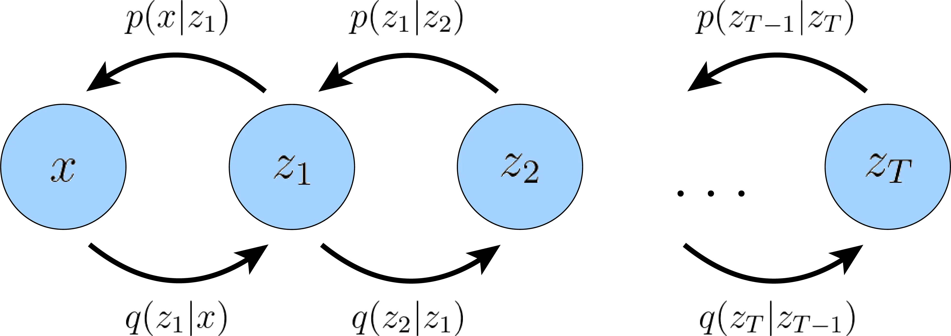
To consider a simple example, take a Markovian chain of VAEs, where each decoding latent variable $z_t$ is dependent on the previous one $z_{t+1}$. This can be simply seen as a recursive stack of VAEs and we can model the joint distribution, and the posterior as:

$$\begin{array}{rl}p(x,z_{1:T})& =p(z_T)p_{\theta }(x|z_1)\prod _{t=2}^T{p}_{\theta }(z_{t-1}|z_t)\\ q_{\varphi }(z_{1:T}|x)& =q_{\varphi }(z_1|x)\prod _{t=2}^T{q}_{\varphi }(z_t|z_{t-1})\end{array}$$

And similarly, ELBO can be extended:

$$\begin{array}{rl}\log p(x)& =\log \int p(x,z_{1:T})d{z}_{1:T}\\ & =\log E_{q_{\varphi }(z_{1:T}|x)}\left[\frac{p(x,z_{1:T})}{q_{\varphi }(z_{1:T}|x)}\right]\\ & \ge E_{q_{\varphi }(z_{1:T}|x)}\left[\log \frac{p(x,z_{1:T})}{q_{\varphi }(z_{1:T}|x)}\right]\end{array}$$

References

• 33  Generative Modeling Meets Representation Learning – Foundations of Computer Vision
• Understanding Diffusion Models: A Unified Perspective
• From Autoencoder to Beta-VAE | Lil’Log
• Eric Jang: A Beginner’s Guide to Variational Methods: Mean-Field Approximation

1. Kingma, D. P., & Welling, M. (2013). Auto-encoding variational bayes. arXiv preprint arXiv:1312.6114.
2. Sønderby, C. K., Raiko, T., Maaløe, L., Sønderby, S. K., & Winther, O. (2016). Ladder variational autoencoders. Advances in neural information processing systems, 29.
3. Kingma, D. P., Salimans, T., Jozefowicz, R., Chen, X., Sutskever, I., & Welling, M. (2016). Improved variational inference with inverse autoregressive flow. Advances in neural information processing systems, 29.