score-matching

Score based generative models

We have shown in VDM that approximating the score function is analogous to predicting the posterior mean ${\mu }_q$ or noise $ϵ$. We can now look at another class of models: Score-based Generative models that directly learn the score function and then sample from the distribution using MCMC methods like Annealed Langevin sampling.

Recall, in EBMs, we represent an arbitrary distribution using Boltzmann energy function, $p_{\theta }(x)=\frac{1}{Z(\theta )}\exp (-f_{\theta }(x))$, where $f_{\theta }$ is arbitrary, flexible and parametrizable function and $Z_{\theta }$ is the normalising or partition function written as $\int \exp (-f_{\theta }(x))dx$. One way to learn such a distribution is Maximum likelihood estimation but requires tackling the constant $Z_{\theta }$ which can be computed using MC estimate of the samples, but that might be difficult to get for complex $f_{\theta }$ functions.

To make likelihood training feasible, models restrict their architectures or approximate normalising constant:

• Causal convolutions in AR models: likelihood is written using chain rule that avoids normalising constant
• Normalising flows: uses change-of-variables to solve the problem differently.
• VAE: Avoid latent variable integral using ELBO maximisation.
• MCMC sampling: approximate expectation using real samples or the current best samples.

Learning the score function using neural network approximation $s_{\theta }$ is one way to avoid modelling the normalisation constant.

$$\begin{array}{rl}{\nabla }_{\mathbf{x}}\log p(\mathbf{x})& ={\nabla }_{\mathbf{x}}\log \exp (-f_{\theta }(\mathbf{x}))-{\nabla }_x\log Z_{\theta }\\ & =-{\nabla }_{\mathbf{x}}{f}_{\theta }(\mathbf{x})\\ & \approx s_{\theta }(\mathbf{x})\end{array}$$

We can then compute the score either by directly modelling the unnormalised energy function $f_{\theta }$ or approximating the score function with a neural network $s_{\theta }$. The neural network is then trained using the fisher divergence measure between estimated score and ground truth score function.

$$\begin{array}{c}{\mathbb{E}}_{p(x)}\left[\Vert s_{\theta }(\mathbf{x})-\nabla \log p(\mathbf{x}){\Vert }_2^2\right]\end{array}$$

Why use fisher divergence and not other divergence measures?

Due to the flexibility of fisher divergence, $s_{\theta }$ doesn’t need to be any normalised distribution, and simply compares the ${\ell }_2$ distance between ground truth score and the learned model.

What does score function mean, what does it represent?

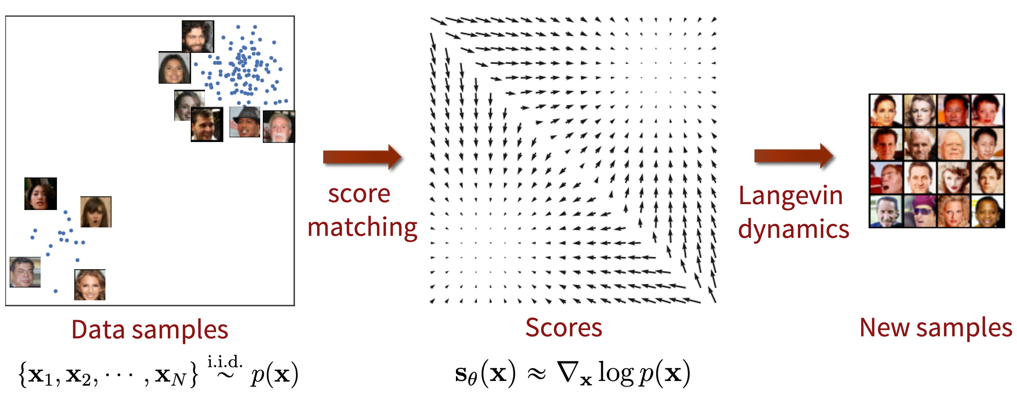
Score function is the gradient of the log likelihood of the data $\mathbf{x}$. Geometrically, it defines a vector field over the space of $x$ pointing towards the peaks.

add a plot for langevin dynamics and score function.

After learning the true distribution by modelling the score function, we can just sample from the distribution. Langevin sampling is an MCMC sampling procedure that enables drawing sample from the distribution using just the score function which we’ve learned as $s_{\theta }$, and arbitrary isotropic Gaussian noise. We update the values and iteratively follow the direction until a mode is reached.

$${\mathbf{x}}_{i+1}\leftarrow {\mathbf{x}}_i+ϵ{\nabla }_{\mathbf{x}}\log p(\mathbf{x})+\sqrt{2ϵ}{\mathbf{z}}_i,i=1,2,\dots ,K$$

and ${\mathbf{z}}_i\sim \mathcal{N}(0,I)$. As $ϵ\to 0$ and $K\to \infty$, the sequence converges to the mode of the distribution. The extra noise term ensures that the procedure is not entirely deterministic and sufficient exploration is performed at each iteration.

For what scenarios, we can have access to the ground truth score function, and for what, do we not have?

In case, we do not have access, we can use score matching techniques to minimise fisher divergence. Combination of learning the score function using score matching, and sampling using langevin dynamics is known as SCGM.

What are the three main problems of vanilla score matching?

• From manifold hypothesis, we know that x lies on a low-dimensional manifold in a high-dimensional space. Computing log of the probability of the points not in low-dimensional manifold is undefined, which means, even if we have access to ground truth score function, it leads to numerical instability errors when learning on low-probability points.
• Model is trying to estimate the expectation of L2 norm of difference between learned score function and ground truth. In low-density regions, where few data points are available, probability assigned to the point will be very low, and model will not gain any significant information from the input. Sampling from Langevin dynamics involves starting from a random point and iteratively following the score. Starting sample is highly likely to be in low-density regions. Due to inaccurate scores in those regions, model may never find the mode, and the final generated sample may be suboptimal.
• Langevin sampling may not consider the weight of the mixture of distributions. Suppose the distribution is p(x)=cp1(x)+c2p2(x). Computing the score using gradient of log probability erases the weight of the distribution. The learned score function may then be agnostic to the different weights, and langevin sampling then leads to a different peak irrespective of the strengths in the combined distribution.

How to mitigate this problem? How can the problem be summed in one sentence? The problem is due to lack of signal in low-density regions. This is equivalent of using an unseen image from the true distribution to the network.

The solution is quite simple, yet elegant, and follows the same process as VDM, i.e. to perturb data points with noise, and train a score based model on the noisy data. This fixes two of the three previously stated problems. Suppose, we perturb a high-dimensional distribution with additional Gaussian noise: $\tilde{x}=x+\sigma z,z\sim \mathcal{N}(0,I)$.

• Due to the support of Gaussian being the entire space, a perturbed sample is no longer confined to high-density region, $p_{\sigma }(x)>0,\forall x$. Mathematically, this is equivalent of taking a convolution with a Gaussian kernel: $p_{\sigma }(\tilde{x})=\int p(x)\mathcal{N}(\tilde{x};x,{\sigma }^{2}I)dx$
• Adding Large Gaussian noise smoothens out the peaks of the distribution more aggressively, and model can get training signal from low-density areas.

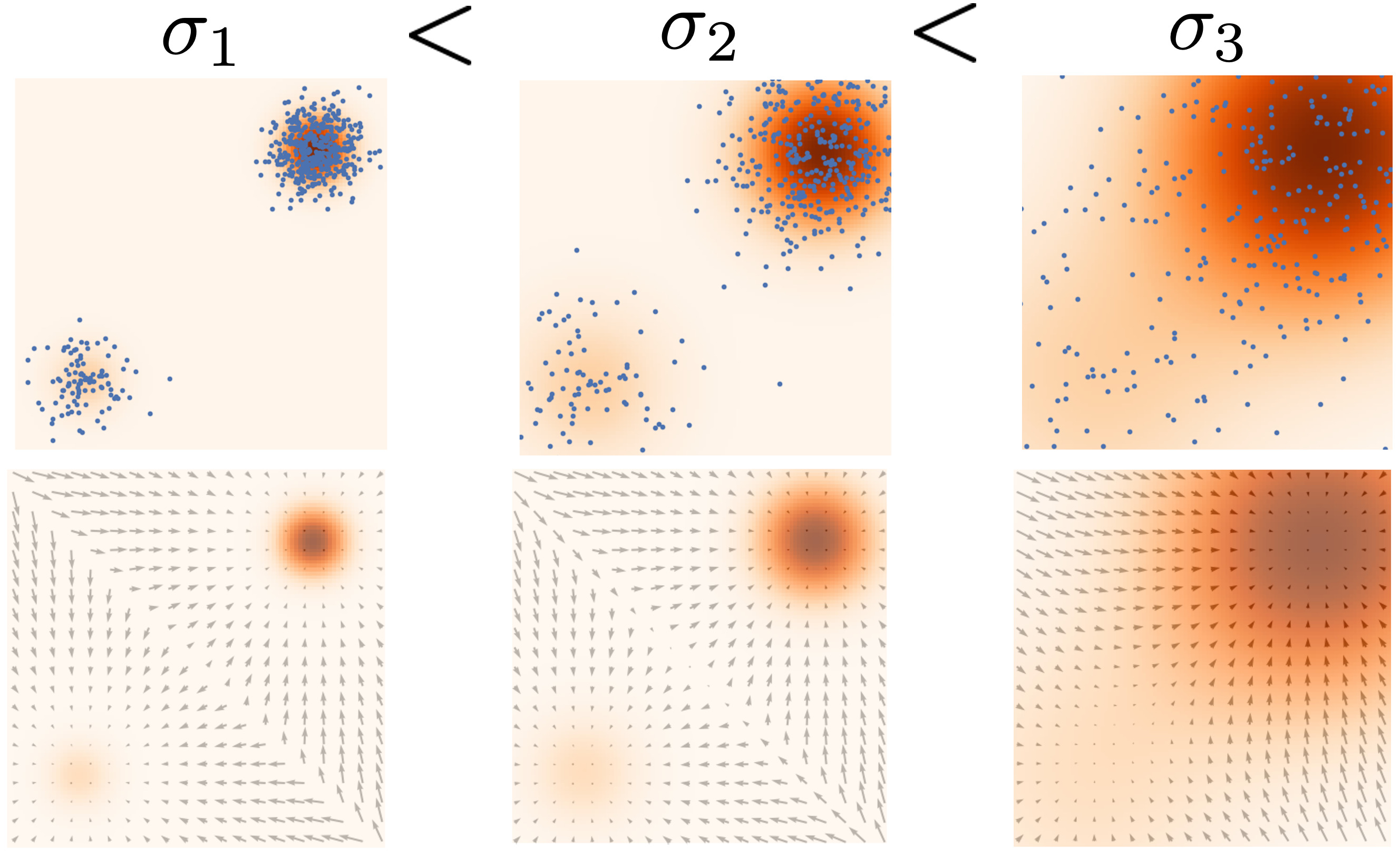
To fix the third problem is a little tricky, because adding single big noise could alter the distribution and the model could potentially be learning an incorrect distribution altogether. The solution to this is actually, quite similar to VDMs again, i.e. add multiple noise at successive levels that result in intermediate distributions. Distributions with smaller noise respect the weighing coefficients in a mixture of distributions while larger noise the model can learn global structure to sufficiently guide the score matching objective.

Suppose, we always perturb the data with isotropic Gaussians.

• Take L Gaussians with increasing standard deviations: ${\sigma }_1<{\sigma }_2<\cdots <{\sigma }_L$.
• Perturb the data distribution $p(x)$ with each of the noisy Gaussian to obtain a sequence of more noisy distributions: $p_{{\sigma }_i}(x)=\int p(z)\mathcal{N}(x;z,{\sigma }_i^{2}I)dz,i=1,2,\dots ,L$
• Drawing samples from each of the distribution is trivial, $x\sim p(x)$, and computing $x+{\sigma }_{i}z,z\sim \mathcal{N}(0,I)$
• Train a neural network approximator to learn the score function for all noise level simultaneously. The objective is a weighted sum of fisher divergences of each noisy distribution $\arg {\min }_{\theta }{\sum }_{t=1}^T\lambda (t){\mathbb{E}}_{p_{{\sigma }_t}(x_t)}\left[\Vert s_{\theta }(x,t)-\nabla \log p_{{\sigma }_t}(x_t){\Vert }_2^2\right]$

After training, produce samples by running Annealed Langevin dynamics which is just Langevin dynamics that runs for each distribution $t=T,T-1,\dots ,1$ in sequence, and initialisation for each sampling is the output of the previous sampler. You can note how the noise reduces with each new sampler, and the most recent sample is used as the initialiser to carry-forward the information learned from previous step. This can be interpreted as reverse diffusion process of a VDM, where an isotropic noisy vector is gradually refined towards lesser noise levels.

Score matching techniques

• Explicit score matching
• Implicit score matching
• Denoising score matching
• sliced score matching

References

• Generative Modeling by Estimating Gradients of the Data Distribution | Yang Song

1. Song, Yang, and Stefano Ermon. “Generative modeling by estimating gradients of the data distribution.” Advances in neural information processing systems 32 (2019).

Score based Generative Modelling using SDEs

Write a table that compares between diffusion and SDE formulation of diffusion and compares forward and reverse process with an SDE.

A quick primer on SDEs

Time reversal of diffusion/reverse SDE

• Why do we want to reverse an SDE? What do we aim to get by tracing back the forward trajectory of an SDE?
  • We can’t trace back the trajectory exactly, and get back the initial position, but what we can do aim is, at initial time $t_0$, the particles should have the position as per the forward SDE’s initial distribution.
  • Or even stronger assumption, at any point t, the position of the particles match the distribution of the forward trajectory.
  • We say that distribution is matched when the probability mass is conserved as the process progresses.
  • Andersen’s theorem provides the solution to reverse an SDE and is mathematically stated as $d\mathbf{x}=[f(\mathbf{x},t)-g(t{)}^2{\nabla }_x\log p_t(\mathbf{x})]dt+g(t)d\bar{\mathbf{w}}$, where $\bar{\mathbf{w}}={\mathbf{w}}_{t-1}-{\mathbf{w}}_t$.

Take an ODE, reverse it using sign change

• sampling methods for ODE
  • first-order method: Euler’s method
  • second-order method: Runge-Kutta

For an SDE,

• sample using euler-maruyama
• reverse using andersen’s theorem
• Ornstein-Uhlenbeck: linear drift + constant diffusion.

We can take the DDPM process and write it in the form of continuous time SDE. To see the process, let’s start with forward diffusion: ${\mathbf{x}}_i=\sqrt{1-{\beta }_i}{\mathbf{x}}_{i-1}+\sqrt{{\beta }_i}{z}_{i-1}$, where $z_i\sim \mathcal{N}(0,I)$. Any iterative process can bee converted into an ODE. For an SDE conversion, we’ll follow similar approach.

For N-step diffusion process:

1. Define a step size $\Delta t=\frac{1}{N}$
2. Consider auxilliary noise level $\{{\bar{\beta }}_i{\}}_{i=1}^N$ where ${\beta }_i=\frac{{\bar{\beta }}_i}{N}$. We define ${\beta }_i$ this way because as ${\lim }_{N\to \infty }\frac{{\bar{\beta }}_i}{N}\approx \beta (t)\Delta t$.
3. Similarly define ${\mathbf{x}}_i=\mathbf{x}\left(\frac{i}{N}\right)=\mathbf{x}(t+\Delta t)$ and ${\mathbf{z}}_i=\mathbf{z}\left(\frac{i}{N}\right)=\mathbf{z}(t+\Delta t)$
4. Following the diffusion process,

$$\begin{array}{rlr}{\mathbf{x}}_i& =\sqrt{1-{\beta }_i}{\mathbf{x}}_{i-1}+\sqrt{{\beta }_i}{z}_{i-1}& \\ x(t+\Delta t)& =\sqrt{1-\beta (t+\Delta t)\Delta t}\mathbf{x}(t)+\sqrt{\beta (t+\Delta t)\Delta t}z(t)& (\text{Putting βi=βˉi/N and substituting})\\ & \approx \left(1-\frac{1}{2}\beta (t+\Delta t)\Delta t\right)\mathbf{x}(t)+\sqrt{\beta (t+\Delta t)\Delta t}z(t)& \\ & \approx \mathbf{x}(t)-\frac{1}{2}\beta (t)\Delta t\mathbf{x}(t)+\sqrt{\beta (t)\Delta t}z(t)& (\text{substituting }\beta (t+\Delta t)\to \beta (t))\end{array}$$

As $\Delta t\to 0$, $z(t)=\mathbf{w}(t+\Delta t)-\mathbf{w}(t)=d\mathbf{w}$

$$\begin{array}{c}d\mathbf{x}=-\frac{1}{2}\beta (t)\mathbf{x}(t)dt+\sqrt{\beta (t)}d\mathbf{w}\end{array}$$

Reverse sampling equation of DDPM can be written as SDE as

$$d\mathbf{x}=-\beta (t)\left[\frac{\mathbf{x}}{2}+{\nabla }_{\mathbf{x}}\log p_t(x)\right]dt+\sqrt{\beta (t)}d\bar{\mathbf{w}}$$

Following similar iterative update scheme, this can be converted into DDPM reverse sampling equation: ${\mathbf{x}}_{i-1}\approx \frac{1}{\sqrt{1-{\beta }_i}}\left[{\mathbf{x}}_i+\frac{{\beta }_i}{2}{\nabla }_{\mathbf{x}}\log p_i({\mathbf{x}}_i)\right]+\sqrt{{\beta }_i}{\mathbf{z}}_i$.

Why DDPM SDE is called Variance-Preserving SDE?

Why SMLD SDE is called Variance exploding SDE?